Kernel methods

I gave this talk on the 27th of May of 2025 for the study group on Machine Learning organised by Marc Truter and Hefin Lambley. It had a theoretical component, where I explained the theory behind kernel methods, and a practical component, where I showed how to implement them using the sklearn library.

Theory

Kernel methods are a powerful set of techniques in machine learning that are used for building non-linear prediction models.

In previous weeks of the study group, we saw how to construct linear models that allow us to find trends in data. However, as we know, most phenomena that machine learning excels at studying, from image recognition to natural language processing, are inherently non-linear.

Kernels provide a way to solve non-linear problems by transforming them into equivalent problems that can be solved efficiently using linear methods.

Let’s start with an example

A very illustrative example is the following:

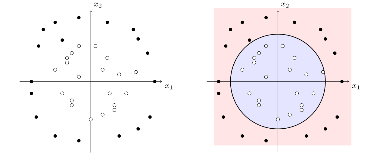
Suppose that we want to build a model that allows us to classify data into two categories, and we have the following training data:

We would like to be able to find a curve in the coordinate plane that splits the plane into two regions, one for each category. In this case, it is quite clear that using a line to separate the data is not going to work well, but it seems like this data could be approximated well by a closed shape, for example, a circle.

Now, here is the trick on how to classify the data. Instead of trying to fit a linear model on the data \((x_1,x_2)\in\mathbb{R}^2\), we generate points in \(\mathbb{R}^5\) of the form \((x_1,x_2,x_1^2,x_1x_2,x_2^2)\) and try to use a hyperplane to separate the data.

Indeed, just by considering \(\{x_1^2,x_2^2\}\), we can easily see that the data can be easily separated with a line:

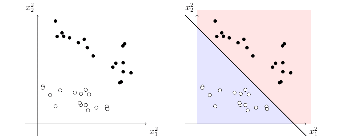
Now, this line corresponds to a conic in the original space, which separates our original data:

This idea of mapping the data into a higher-dimensional space is the essence of kernel methods. In the exercise session, we will see how to implement them in practice using the sklearn library. But let’s first explain the theory behind the kernel approach.

Theoretical background

As in the past, let \((x_i,y_i)\in\mathcal{X}\times\mathcal{Y}\) be a set of training data of size \(n\), where \(\mathcal{X}\subseteq\mathbb{R}^d\) is the input space and \(\mathcal{Y}\) is the output space. Our goal is to learn a function \(f\colon\mathcal{X}\to\mathcal{Y}\) that approximates the relationship between the inputs and outputs.

For today’s talk, we will focus on the case where \(\mathcal{Y}=\{-1,1\}\), which is the case of binary classification. As \(\mathcal{Y}\) is discrete, what we do instead is that we learn a function \(f_\theta\colon\mathcal{X}\to\mathbb{R}\) and then, we set \(f(x)=\text{sign}(f_\theta(x))\). This function \(f_\theta\) is called the prediction function, and we will assume that it is a linear function on some parameters \(\{\theta_1,\dots,\theta_m\}\). Assume we also have a loss function \(\ell\colon\mathcal{Y}\times\mathbb{R}\to\mathbb{R}\) that measures how well the prediction function \(f_\theta\) fits the data. For example, we can consider the square loss \(\ell(y,f_\theta(x))=(y-f_\theta(x))^2\).

Let us now choose a function \(\varphi\colon\mathcal{X}\rightarrow\mathbb{R}^m\) that maps the input space \(\mathcal{X}\) to a different space \(\mathbb{R}^m\). This is what we will call the feature map.

Going back to our example, there, we defined the feature map to be

and the function we are trying to learn is \(f_\theta(x_1,x_2)=\theta_1 x_1^2 + \theta_2 x_2^2+\theta_3\), for some parameters \(\theta_1,\theta_2,\theta_3\in\mathbb{R}\). If we denote by \((x_i,y_i)\) our data, we can write \(f_\theta(x_i)\) in terms of the usual inner product as \(f_\theta(x_i)=\langle\theta, \varphi(x_i)\rangle\). We would like to find the parameter \(\theta=(\theta_1,\dots,\theta_m)\in\mathbb{R}^m\) that minimises what is known as the empirical risk:

The first term of this expression represents how close the \(f_\theta(x_i)\) are to the correct values in our training data, whereas \(\frac{\lambda}{2}\lVert \theta\rVert^2\) is a regularization term that prevents overfitting by penalizing large values of the parameter \(\theta\). We can use linear regression to find the parameter \(\theta\) that minimises this expression.

Introducing kernels

From the discussion above, we saw that we can reduce non-linear problems to linear ones by using a feature map \(\varphi\). In practice, there are two issues with this approach:

• We often do not know how to choose a good feature map \(\varphi\) and we may need to try several ones before finding one that works well.
• Solving the optimisation problem above can be computationally expensive, especially if the input data has very large dimension. This is something common in many problems, particularly, when we have very sparsely populated data.

To model mathematically how it is to work with very high dimensional data, we can use Hilbert spaces. Recall that a Hilbert space is a vector space \(\mathcal{H}\) (possibly of infinite dimension) with an inner product space that is complete with respect to the norm induced by the inner product.

Assume that the feature map \(\varphi\) now takes values in \(\mathcal{H}\) rather than \(\mathbb{R}^{m}\). One would imagine that solving the optimisation problem given by \((1)\) in this setting is now even more difficult, as we may be working in a space with infinite dimension. But there is a theorem that guarantees that the difficulty of the problem only depends on the number of elements in our training data, not on the size of the input space \(\mathcal{X}\):

Representer Theorem (for supervised learning). For \(\lambda>0\), the infimum of the empirical risk

can be obtained by restricting to a vector \(\theta\) of the form:

where \(\alpha=(\alpha_1,\dots,\alpha_n)\in\mathbb{R}^n\).

Now, let us define the kernel function \(k\) induced by the feature map \(\varphi\) to be

Let \(K \in \mathbb{R}^{n \times n}\) be the kernel matrix whose entries are given by \(K_{ij}=k(x_i,x_j)\). Then, if we have \(\theta=\sum_{i=1}^n \alpha_i \varphi(x_i)\),

and

so that we can rewrite the optimisation problem as

This what is known as the kernel trick: instead of working with the feature map \(\varphi\), we can work directly with the kernel matrix \(K\). This allows us to work with high-dimensional data without having to explicitly compute the feature map \(\varphi\).

As a matter of fact, we can forget about the feature map \(\varphi\) altogether and just work with the kernel function \(k\), for the following reason:

We say that a function \(k \colon \mathcal{X} \times \mathcal{X} \to \mathbb{R}\) is a positive-definite kernel if, for any finite set of points \(x_1,\dots,x_n\in\mathcal{X}\), the kernel matrix \(K\) restricted to those points is symmetric positive semi-definite. Then, we have this theorem:

Theorem (Aronszajn, 1950) The function \(k:\mathcal{X}\times\mathcal{X}\to\mathbb{R}\) is a positive-definite kernel if and only if there exists a Hilbert space \(\mathcal{H}\) and a function \(\varphi:\mathcal{X}\rightarrow\mathcal{H}\) such that for all \(x,x'\in\mathcal{X}\), \(k(x,x')=\langle \varphi(x),\varphi(x')\rangle\).

Therefore, the existence of a kernel function \(k\) is equivalent to the existence of a feature map \(\varphi\) in some Hilbert space. For any positive-definite kernel \(k\), the space that we build from the kernel is called the reproducing kernel Hilbert space (RKHS).

There are many other reasons why working with kernels is useful, including the fact that there are very efficient algorithms to compute kernels and solve their optimisation problem.

Examples of kernels

There are many different kernels that can be used in practice. Some of the most common ones are:

• Linear kernel: \(k(x,x')=x^\top x'\), \(\forall x,x'\in\mathcal{X}\subseteq\mathbb{R}^d\). Here, the kernel trick can be useful when the input data have huge dimension \(d\), but is quite sparse, such as in text processing.

• Polynomial kernel: \(k(x,x')=(1+x^\top x')^s\), \(\forall x,x'\in\mathcal{X}\subseteq\mathbb{R}^d\). The image of the feature map is the set of all polynomials on \(d\) variables of degree at most \(s\).

• Homogeneous polynomial kernel: \(k(x,x')=(x^\top x')^s\), \(\forall x,x'\in\mathcal{X}\subseteq\mathbb{R}^d\). The image of the feature map is the set of degree \(s\) homogeneous polynomials on \(\mathbb{R}^d\).

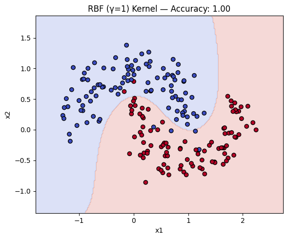
• Radial basis function (RBF) kernel: \(k(x,x')=\exp\left(-\gamma\lVert x-x'\rVert^2\right)\), \(\forall x,x'\in\mathcal{X}\subseteq\mathbb{R}^d\). This kernel is also known as the Gaussian kernel, and it is particularly useful in many applications, such as image processing and natural language processing. The parameter \(\gamma>0\) controls the boundary of the decision region, in the sense that as \(\gamma\) grows, the boundary becomes more complicated and can fit the data better, but it also increases the risk of overfitting.

• Translation invariant kernels: \(k(x,x')=q(x-x')\), \(\forall x,x'\in[0,1]\). The idea behind this class of kernels is that the space of square-integrable functions on \([0,1]\) is a Hilbert space with the inner product given by \(\langle f,g\rangle=\int_0^1 f(x)g(x)\,dx\). An orthonormal basis of \(L_2([0, 1])\) is given by the functions \(\sin(2\pi m x)\) and \(\cos(2\pi n x)\) for \(m,n\in\mathbb{N}\), and we can study many aspects of \(q(x)\) from the perspective of Fourier analysis. These kernels are particularly useful in time series analysis, where we can use them to study periodic phenomena (e.g., weather patterns, seasonal financial trends…)

We will now see how to work with some of these kernels in practice in the exercise session.

Practice

In this practical session, we are going to be coding the problem that we discussed at the start of the talk: how to use kernels to solve non-linear classification problems.

The techniques used to divide a set of observations in the decision space using hyperplanes are usually referred to as Support Vector Machines (abbreviated as SVMs). The reason why they are called that way is because what they do is to maximise the distance of the hyperplane to the support vectors, which are the data points that are closest to the decision surface.

Learning how to use SVMs in Python

We start by importing the libraries that we will need for this exercise:

# Imports
import numpy as np
import matplotlib.pyplot as plt
from sklearn.datasets import make_moons
from sklearn.svm import SVC
from sklearn.model_selection import train_test_split
from sklearn.metrics import accuracy_score

Now, we are going to generate the data that we will use for the exercise. We will use the make_moons function from sklearn.datasets, which generates a two-dimensional dataset with a non-linear decision boundary.

# Generate synthetic 2D data (nonlinear)
X, y = make_moons(n_samples=200, noise=0.2, random_state=13)
X_train, X_test, y_train, y_test = train_test_split(
    X, y, test_size=0.2, random_state=42
)  # We use the train_test_split function to split the dataset into training and testing sets.

The function SVC from sklearn.svm implements the Support Vector Machine algorithm. It takes as arguments the kernel to be used, the regularisation parameter \(C\), and the degree of the polynomial kernel if it is used. The regularisation parameter \(C\) is related to the \(\lambda\) that we explained in the talk and controls the trade-off between maximizing the margin, which is the distance to the support vectors and minimising the classification error. A small value of \(C\) will result in a larger margin but may misclassify some points, while a large value of \(C\) will result in a smaller margin but will classify all points correctly.

# Here are some examples of SVM kernels that can be used for classification tasks:
kernels = {
    "Linear": SVC(kernel="linear", C=1),
    "Polynomial (degree=7)": SVC(kernel="poly", degree=7, C=1),
    "RBF (γ=1)": SVC(kernel="rbf", gamma=1, C=1),
}

Recall that we use fit to train the model and predict to make predictions. We can compute the accuracy of the model by comparing the predicted labels with the true labels using the accuracy_score function from sklearn.metrics.

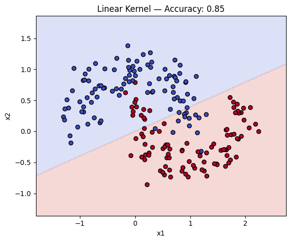
# We see that the accuracy of the linear kernel is 85%
linkernel = SVC(kernel="linear", C=1)
linkernel.fit(X_train, y_train)
y_pred = linkernel.predict(X_test)
acc = accuracy_score(y_test, y_pred)
print(acc)

Let’s now plot the decision boundary of the SVM model. We will create a plot_decision_boundary function to visualize the decision boundary.

# Plot decision boundary
def plot_decision_boundary(ker, X, y, title):
    h = 0.02
    x_min, x_max = X[:, 0].min() - 0.5, X[:, 0].max() + 0.5
    y_min, y_max = X[:, 1].min() - 0.5, X[:, 1].max() + 0.5
    xx, yy = np.meshgrid(np.arange(x_min, x_max, h), np.arange(y_min, y_max, h))
    Z = ker.predict(np.c_[xx.ravel(), yy.ravel()])
    Z = Z.reshape(xx.shape)

    plt.figure(figsize=(6, 5))
    plt.contourf(xx, yy, Z, alpha=0.2, cmap=plt.cm.coolwarm)
    plt.scatter(X[:, 0], X[:, 1], c=y, cmap=plt.cm.coolwarm, edgecolors="k")
    plt.title(title)
    plt.xlabel("x1")
    plt.ylabel("x2")
    plt.tight_layout()
    plt.show()

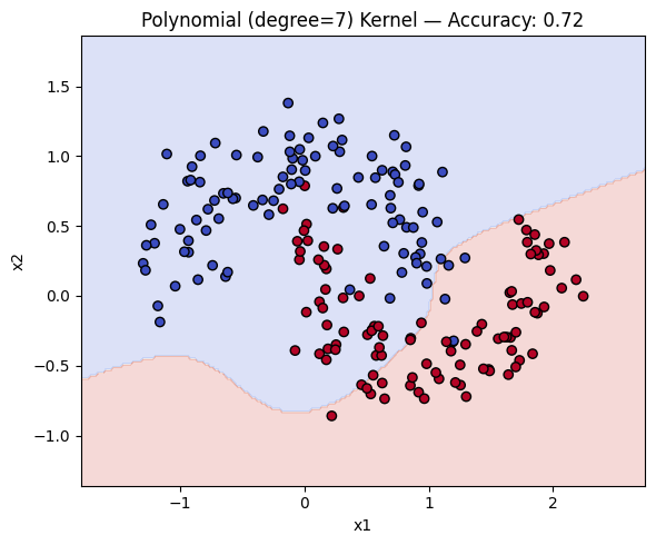
Now, we can compare how the three types of kernels compare in terms of accuracy and decision boundary.

for name, ker in kernels.items():
    ker.fit(X_train, y_train)
    y_pred = ker.predict(X_test)
    acc = accuracy_score(y_test, y_pred)
    plot_decision_boundary(ker, X, y, f"{name} Kernel — Accuracy: {acc:.2f}")

Now it’s your turn!

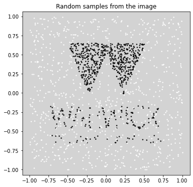
For this exercise session, we are going to compute the decision boundary of a Support Vector Machine using different kernels. We are going to generate the data from a picture. In this case, our image is the Warwick logo, and we are going to sample the points according to whether they are black or white pixels in the image. Feel free to use any image you like!

Note: To work with images, we’ll use the scikit-image package, which we import using the name skimage. As in talk 1, you can install this using the pip package manager (for most users, just type pip install scikit-image in your terminal, just like we did at the start of the reading group).

from skimage import io, color
from skimage.filters import gaussian

# Load image
img = io.imread("warwick.jpg")  # should be a black-and-white silhouette
plt.imshow(img)
plt.axis("off")
plt.title("Original Image")
plt.show()

# Convert to grayscale
gray = color.rgb2gray(img)

# Apply Gaussian blur so the edges are not too sharp
gray = gaussian(gray, sigma=1)

# Threshold to get a binary mask
threshold = 0.3
maskb = gray < threshold  # black = foreground
maskw = gray > 1 - threshold  # white = foreground

# Get coordinates of black pixels
coordsb = np.column_stack(np.where(maskb))
coordsw = np.column_stack(np.where(maskw))

# Rescale both coordsb and coordsw to the same [-1, 1] square using global min/max
all_coords = np.vstack([coordsb, coordsw]).astype(float)
min0, max0 = all_coords[:, 0].min(), all_coords[:, 0].max()
min1, max1 = all_coords[:, 1].min(), all_coords[:, 1].max()

coordsb = coordsb.astype(float)
coordsw = coordsw.astype(float)
coordsb[:, 0] = 2 * (coordsb[:, 0] - min0) / (max0 - min0) - 1
coordsb[:, 1] = 2 * (coordsb[:, 1] - min1) / (max1 - min1) - 1
coordsw[:, 0] = 2 * (coordsw[:, 0] - min0) / (max0 - min0) - 1
coordsw[:, 1] = 2 * (coordsw[:, 1] - min1) / (max1 - min1) - 1

# The orientation is questionable, so we flip the axes
dum = coordsb.copy()
coordsb[:, 0] = dum[:, 1]
coordsb[:, 1] = -1 * dum[:, 0]
dum = coordsw.copy()
coordsw[:, 0] = dum[:, 1]
coordsw[:, 1] = -1 * dum[:, 0]

# Subsample randomly from both sets of coordinates
n_points = 800  # This is the number of points to sample from each set
idxb = np.random.choice(len(coordsb), size=n_points, replace=False)
idxw = np.random.choice(len(coordsw), size=n_points, replace=False)
XB = coordsb[idxb]
XW = coordsw[idxw]

# Visualise
plt.figure(figsize=(6, 6))
plt.scatter(XB[:, 0], XB[:, 1], s=2, color="black")  # note flipped axes
plt.scatter(XW[:, 0], XW[:, 1], s=2, color="white")  # note flipped axes
plt.title("Random samples from the image")
plt.axis("equal")
plt.gca().set_facecolor("lightgray")  # or any color you prefer, e.g. "#f0f0f0"
plt.show()

Exercises

Exercise 1

Now that we have generated the data, let’s try to train the models. We have two arrays, XB and XW that contain the coordinates of the black and white pixels, respectively. Your first task is to produce training and testing sets from these arrays. You can use the train_test_split function from sklearn.model_selection to do this. It takes as arguments two arrays \(X\) with the data and \(y\) with the labels of $$X$; the test size, and a random state (that is used for reproducibility).

To compute \(X\) and \(y\), you may find useful to use the following functions:

• np.vstack and np.hstack can be used to stack arrays vertically and horizontally, respectively.
• np.zeros and np.one can be used to produce arrays of length \(n\) with only zeros or ones, respectively.

# Create training data from XB (label 0) and XW (label 1)
X = __
print(X)
y = __
print(y)
X_train, X_test, y_train, y_test = train_test_split(X, y, test_size=__, random_state=__)

Exercise 2

Let’s now compare how different kernels perform on this dataset. More specifically, we will compare how does the polynomial kernel perform with different degrees. First, we will create a dictionary containing all polynomial kernels of degrees from 1 to 9.

More specifically, what I want is a dictionary whose keys are “Polynomial of degree d” and the values are the SVM models with the polynomial kernel of degree \(d\), with \(d\) ranging from 1 to 9.

# Create a dictionary of polynomial kernels with different degrees.
polykernels = {"__": SVC(kernel="__", degree=__) for d in __}
print(polykernels)

Exercise 3

Let’s do a table with the accuracy of each model. You can use the pandas library to create a data frame with the results. The data frame should have two columns: “Kernel” and “Accuracy”. The “Kernel” column should contain the name of the kernel, and the “Accuracy” column should contain the accuracy of the model.

# Create a data frame to store the name and accuracy of each kernel.
import pandas as pd

results = __
for name, ker in polykernels.items():
    __.fit(__, __)  # Fit the model
    y_pred = __.predict(__)  # Predict the labels for the test set
    acc = accuracy_score(__, __)  # Compute the accuracy
    results.append(
        {"Kernel": __, "Accuracy": __}
    )  # Add starting rows of the data frame
df_results = pd.DataFrame(__)
print(__)

Exercise 4

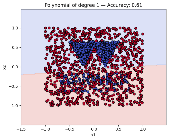
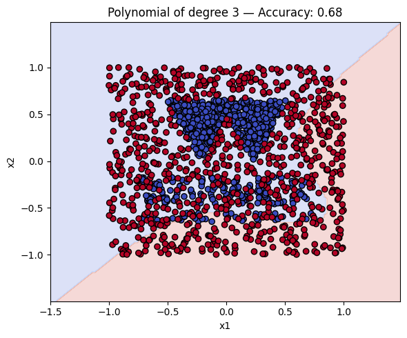
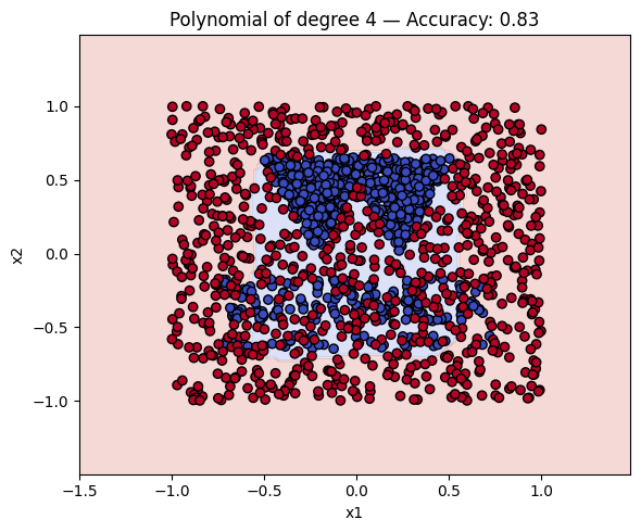
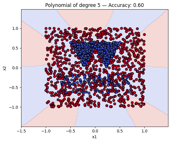
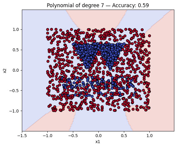
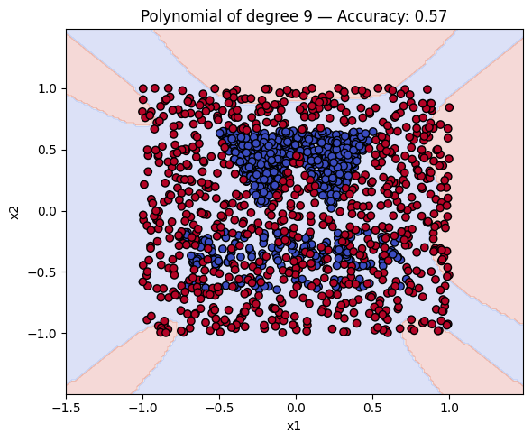
Finally, we will plot the decision boundaries of the models in the dictionary. You can use the plot_decision_boundary function that we defined earlier to do this.

# Make a plot with the decision boundaries of each of the polynomial kernels that includes the name and the accuracy.
for name, ker in polykernels.items():
    ker.fit(__, __)
    y_pred = ker.predict(__)
    acc = accuracy_score(__, __)
    plot_decision_boundary(ker, X, y, f"{__} — Accuracy: {__:.2f}")

Finally, a geometric question to reflect on: why do you think the kernels with even degrees perform better than the kernels with odd degrees? What is the reason behind this?

You can also experiment with the different kernels and see how they perform on the dataset. You can also try to change the regularisation parameter \(C\) and see how it affects the decision boundary.

Solutions

Solution to Exercise 1

# Create training data from XB (label 0) and XW (label 1)
X = np.vstack([XB, XW])
print(X)
y = np.hstack([np.zeros(len(XB)), np.ones(len(XW))])
print(y)
X_train, X_test, y_train, y_test = train_test_split(
    X, y, test_size=0.2, random_state=42
)

Output:

[[-0.33641618  0.31278891]
 [-0.60924855 -0.24191063]
 [ 0.0982659   0.51617874]
 ...
 [ 0.97456647 -0.14021572]
 [ 0.90520231 -0.13097072]
 [ 0.49364162  0.15562404]]
[0. 0. 0. ... 1. 1. 1.]

Solution to Exercise 2

# Create a dictionary of polynomial kernels with different degrees
polykernels = {
    f"Polynomial of degree {d}": SVC(kernel="poly", degree=d) for d in range(1, 10)
}
print(polykernels)

Output:

{'Polynomial of degree 1': SVC(degree=1, kernel='poly'), 'Polynomial of degree 2': SVC(degree=2, kernel='poly'), 'Polynomial of degree 3': SVC(kernel='poly'), 'Polynomial of degree 4': SVC(degree=4, kernel='poly'), 'Polynomial of degree 5': SVC(degree=5, kernel='poly'), 'Polynomial of degree 6': SVC(degree=6, kernel='poly'), 'Polynomial of degree 7': SVC(degree=7, kernel='poly'), 'Polynomial of degree 8': SVC(degree=8, kernel='poly'), 'Polynomial of degree 9': SVC(degree=9, kernel='poly')}

Solution to Exercise 3

import pandas as pd

results = []
for name, ker in polykernels.items():
    ker.fit(X_train, y_train)
    y_pred = ker.predict(X_test)
    acc = accuracy_score(y_test, y_pred)
    results.append({"Kernel": name, "Accuracy": acc})
df_results = pd.DataFrame(results)
print(df_results)

Output:

    Kernel                  Accuracy
0   Polynomial of degree 1  0.606250
1   Polynomial of degree 2  0.809375
2   Polynomial of degree 3  0.678125
3   Polynomial of degree 4  0.831250
4   Polynomial of degree 5  0.603125
5   Polynomial of degree 6  0.834375
6   Polynomial of degree 7  0.593750
7   Polynomial of degree 8  0.815625
8   Polynomial of degree 9  0.571875

Solution to Exercise 4

# Make a plot with the decision boundaries of each of the polynomial kernels that includes the name and the accuracy.
for name, ker in polykernels.items():
    ker.fit(X_train, y_train)
    y_pred = ker.predict(X_test)
    acc = accuracy_score(y_test, y_pred)
    plot_decision_boundary(ker, X, y, f"{name} — Accuracy: {acc:.2f}")